Extracting top 20 words from text
01 Jun 2020
In this post we will use wordcloud() to explore the most frequent words in a text. I suppose you might have come across a figure of cloud filled with bunch of words. You might have also noticed that the words displayed shown in different sizes. The size in turn represent the frequency or the importance of each word. This is called Tag Cloud or WordCloud.
For this purpose we are going to use the 12dancingprincesses.txt file. Open the file and read it, then we use the NLTK library to tokenize each word in the text. After loading and tokenizing each word, we then remove the punctuation and filler words (stopwords) from the list of tokens. At the end we will visualize the top 10 words from the text.
import pandas as pd
import nltk
from nltk.tokenize import word_tokenize
from nltk.tokenize import sent_tokenize
from nltk.tokenize import TweetTokenizer
from nltk.probability import FreqDist
from nltk.corpus import stopwords
from nltk.stem import WordNetLemmatizer
from nltk.sentiment.vader import SentimentIntensityAnalyzer

from nltk.corpus import names
import numpy as np
from string import punctuation
from PIL import Image
#if the next cell does not work #remove number symbol on following lines and re-run this cell
nltk.download(‘punkt’) nltk.download(‘wordnet’) nltk.download(‘names’) nltk.download(‘stopwords’) nltk.download(‘vader_lexicon’)
Tokenizing Words and Sentences
One common task in NLP (Natural Language Processing) is tokenization. Tokens are usually individual words and tokenization is taking a text and breaking it up into individualized words. These tokens are then used as the input for other types of analysis or tasks.
Recall we can use the .split() function to break a sentence apart. In Python tokenization basically refers to splitting up a larger body of text into smaller lines, words or even creating words for a non-English language. The various tokenization functions in-built into the nltk module itself and can be used in programs as shown below.
with open ('datasets/12dancingprincesses.txt',  encoding='cp1252') as file:
    tknz_wct = word_tokenize(file.read().lower())

tknz_wct[:20]
['the',
 'twelve',
 'dancing',
 'princesses',
 'there',
 'was',
 'a',
 'king',
 'who',
 'had',
 'twelve',
 'beautiful',
 'daughters',
 '.',
 'they',
 'slept',
 'in',
 'twelve',
 'beds',
 'all']
What is the length of the tokenized file, what does the distribution look like?
len(tknz_wct)
1849
#the NLTK FreqDist gives a count for how often each part of the text occurs
fd_wct = FreqDist(tknz_wct)
fd_wct
FreqDist({'the': 139, ',': 102, 'and': 78, 'to': 42, '.': 35, ';': 35, 'he': 33, 'they': 32, 'of': 28, '’': 27, ...})
#shows the top 10 words in the text
fd_wct.most_common(10)
[('the', 139),
 (',', 102),
 ('and', 78),
 ('to', 42),
 ('.', 35),
 (';', 35),
 ('he', 33),
 ('they', 32),
 ('of', 28),
 ('’', 27)]
Note here that, the most common parts of this text seem to be filler words and punctuation. We need to remove them to get a better understand of what the text is about.
#number of tokens in list before puntuation removal
len(tknz_wct)
1849
punctuation
'!"#$%&\'()*+,-./:;<=>?@[\\]^_`{|}~'
Notice here that as the punctuations “’” and “‘” are not included we have to add them manually and update the punctuation list.
#if we want to add the quotation mark at the end of
#the wc_tex paragraph use the following
new_punct = punctuation + "’" + "‘"
new_punct
'!"#$%&\'()*+,-./:;<=>?@[\\]^_`{|}~’‘'
#remove the puntuation tokens from the list
for token in tknz_wct:
    if token in punctuation:
        tknz_wct.remove(token)
#number of tokens in list after puntuation removal
len(tknz_wct)
1663
#list of english stopwords
eng_stopwords = stopwords.words('english')
eng_stopwords
['i',
 'me',
 'my',
 'myself',
 'we',
 'our',
 'ours',
 'ourselves',
 'you',
 "you're",
 "you've",
 "you'll",
 "you'd",
 'your',
 'yours',
 'yourself',
 'yourselves',
 ...]
So we added our stop words, updated our punctuation list, thereby removing them we now look for new set of words list.
rm_count = 0
new_words = []  #list to hold new words

for token in tknz_wct:
    if token not in eng_stopwords:
        new_words.append(token)
    else: rm_count += 1
rm_count
944
len(new_words)
719
Now let’s see the new top 10 words in this text. Bear in mind although we have updated our punction list, we have delebarately put it in a different variable name so that means we will expect to still see the two weird quatation marks we have updated.
fd_nw = FreqDist(new_words)
fd_nw.most_common(10)
[('’', 27),
 ('‘', 21),
 ('soldier', 19),
 ('princesses', 17),
 ('said', 16),
 ('king', 15),
 ('twelve', 11),
 ('went', 11),
 ('came', 10),
 ('eldest', 10)]
#if we want to add the quotation mark at the end of
#the wc_tex paragraph use the foooowing
new_punct = punctuation + "’" + "‘"
new_punct
'!"#$%&\'()*+,-./:;<=>?@[\\]^_`{|}~’‘'
make sure to use new_punct instead of punctuation as it consists the new list of updated punctuations, after removing let us redo our counting of new words again.
#remove the puntuation tokens from the list
for token in tknz_wct:
    if token in new_punct:
        tknz_wct.remove(token)
rm_count = 0
new_words = []  #list to hold new words

for token in tknz_wct:
    if token not in eng_stopwords:
        new_words.append(token)
    else: rm_count += 1
#number of tokens in list after puntuation removal
len(tknz_wct)
1618
Therefore now we have the top ten words that doesnt involve the inclusion of common stop words and/or punctuations.
fd_top10 = FreqDist(new_words)
fd_top10.most_common(20)
[('soldier', 19),
 ('princesses', 17),
 ('said', 16),
 ('king', 15),
 ('twelve', 11),
 ('went', 11),
 ('came', 10),
 ('eldest', 10),
 ('one', 7),
 ('night', 7),
 ('happened', 7),
 ('time', 7),
 ('youngest', 7),
 ('bed', 6),
 ('danced', 6),
 ('shoes', 5),
 ('put', 5),
 ('soon', 5),
 ('cup', 5),
 ('princess', 5)]
Visualizig top ten words by wordcloud() and hist()
I usually prefer to visualize results as it shows you clearly relationship that would otherwise would have been missed. It also help reader make sense of what the data is revealing without worrying about the details.
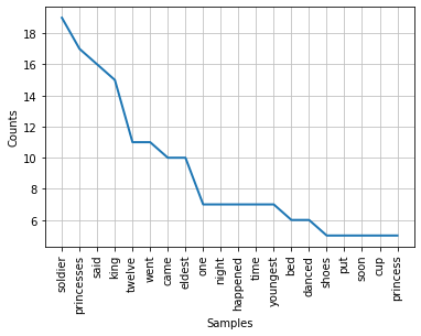
A simple line graph as shown below gives ample information for a quick look. You can see that the plot shows the occurence frequency for top 20 words in decreasing order as we go from soldier to princess (shown on the x-axis). It is a very simple plot yet provides the desired answer. We will see below other options.
%matplotlib inline
fd_top10.plot(20);
Let us now convert the list into dataframe, and add header to the columns. This time we arenot going to sort it and see what the visualization looks like.
#in case you want column header add , columns = ["Word","Frequency"]
df_fdist=pd.DataFrame(list(fd_top10.items()), columns = ["Word","Frequency"])
#df_fdist.sort_values(by="Frequency", ascending=False)
#df_fdist = df_fdist.reset_index(drop=True)
df_fdist
| Word | Frequency | |
|---|---|---|
| 0 | twelve | 11 |
| 1 | dancing | 3 |
| 2 | princesses | 17 |
| 3 | king | 15 |
| 4 | beautiful | 1 |
| ... | ... | ... |
| 351 | eldest. | 1 |
| 352 | married | 1 |
| 353 | day | 1 |
| 354 | chosen | 1 |
| 355 | heir | 1 |
356 rows × 2 columns
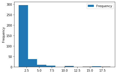
df_fdist.plot(kind='hist')
<matplotlib.axes._subplots.AxesSubplot at 0x7fce86fb2d90>
To see a different version of graphing, let us now make our visualization in barchart, and recall the df is not sorted.
df_fdist_10 =df_fdist.head(20)


ax=df_fdist_10.plot.bar(x='Word',y='Frequency', color='r',figsize=(15,10), title='Top 20 frequent words')
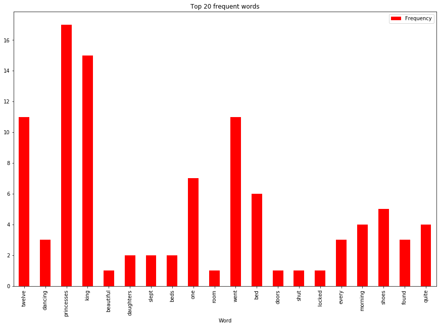
The barchart is interesting even without sorting, one can tell (with a little effort), by looking at the graph, which word is most frequent and which is least frequent.
Another form of visualization is wordcloud. In this case we indicate the frequency of the word by font size, i.e. the bigger the size the most frequent the word is.
We use pythons wordcloud library tl achieve our target. As a preparation because name of header of the columns can be considerd as a word initself we need to make sure to exclude it form the list.
df_fdist_wc = pd.DataFrame.from_dict(fd_top10, orient='index')
df_fdist_wc.columns = ['Frequency']
df_fdist_wc.index.name = 'Term'
print(df_fdist_wc.sort_values(by='Frequency',ascending=False).head(20))
            Frequency
Term
soldier            19
princesses         17
said               16
king               15
twelve             11
went               11
eldest             10
came               10
one                 7
time                7
happened            7
youngest            7
night               7
bed                 6
danced              6
put                 5
lake                5
cup                 5
princes             5
shoes               5
To make it an example let us leave the header as it is, meaning we arenot going to exclude it from the list. On the next cell we will exclude it and see the difference.
from wordcloud import WordCloud, STOPWORDS
import matplotlib.pyplot as plt
text = df_fdist_wc.sort_values(by='Frequency',ascending=False).head(20)


wordcloud = WordCloud(
    width = 1000,
    height = 500,
    background_color = 'black'
    ).generate(str(text))
fig = plt.figure(
    figsize = (40, 30),
    facecolor = 'k',
    edgecolor = 'k')
plt.imshow(wordcloud, interpolation = 'bilinear')
plt.axis('off')
plt.tight_layout(pad=0)
plt.show()
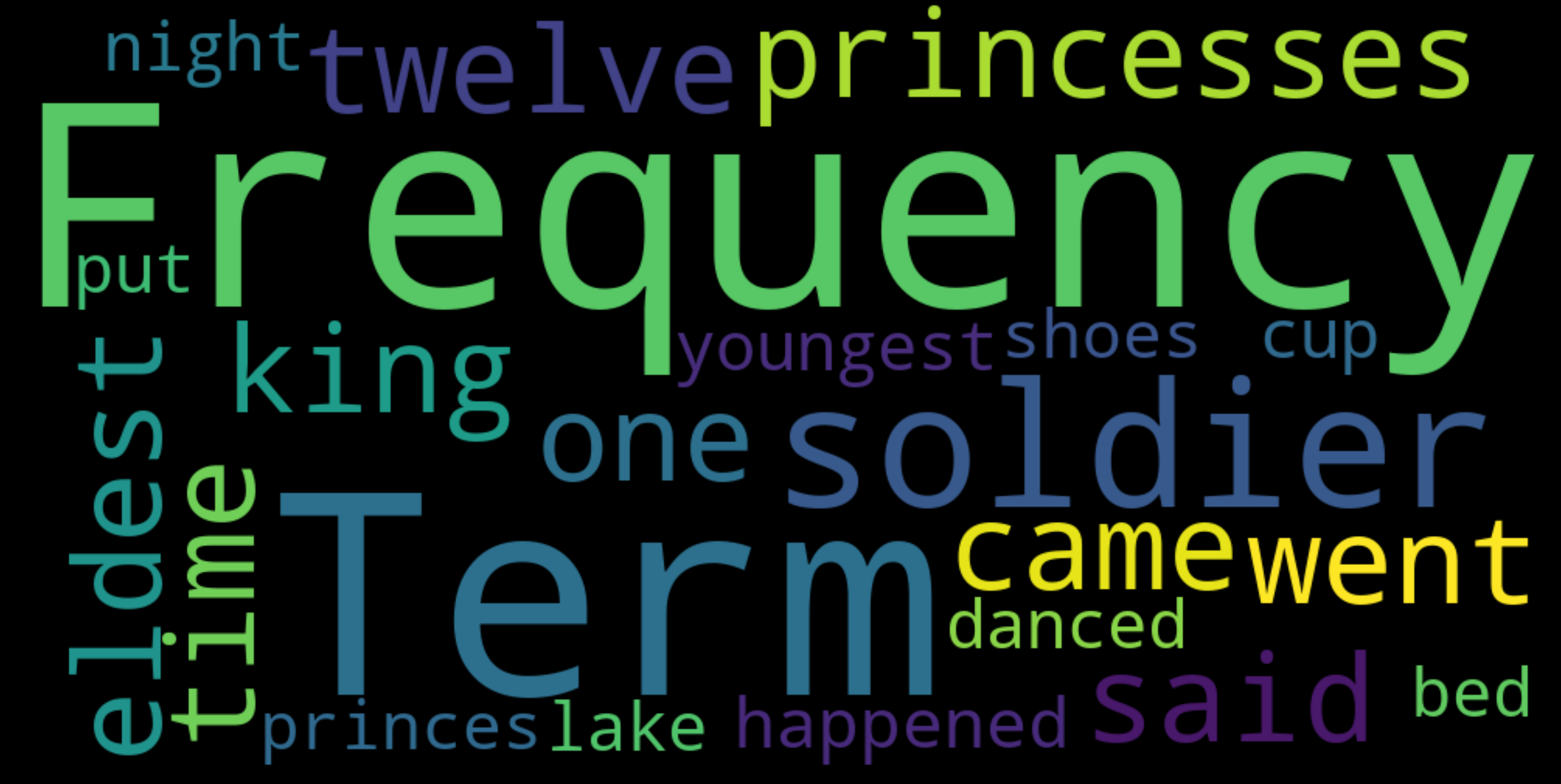
You can see that the column names Frequency and Term dominated the wordcloud, and this is remedied below by adding Frequency and Term into our stopwords, so that the code ignores these two words.
from wordcloud import WordCloud, STOPWORDS
import matplotlib.pyplot as plt
text = df_fdist_wc.sort_values(by='Frequency',ascending=False).head(20)


wordcloud = WordCloud(
    width = 1000,
    height = 500,
    background_color = 'black',
    stopwords =["Term", "Frequency"]).generate(str(text))
fig = plt.figure(
    figsize = (40, 30),
    facecolor = 'k',
    edgecolor = 'k')
plt.imshow(wordcloud, interpolation = 'bilinear')
plt.axis('off')
plt.tight_layout(pad=0)
plt.show()
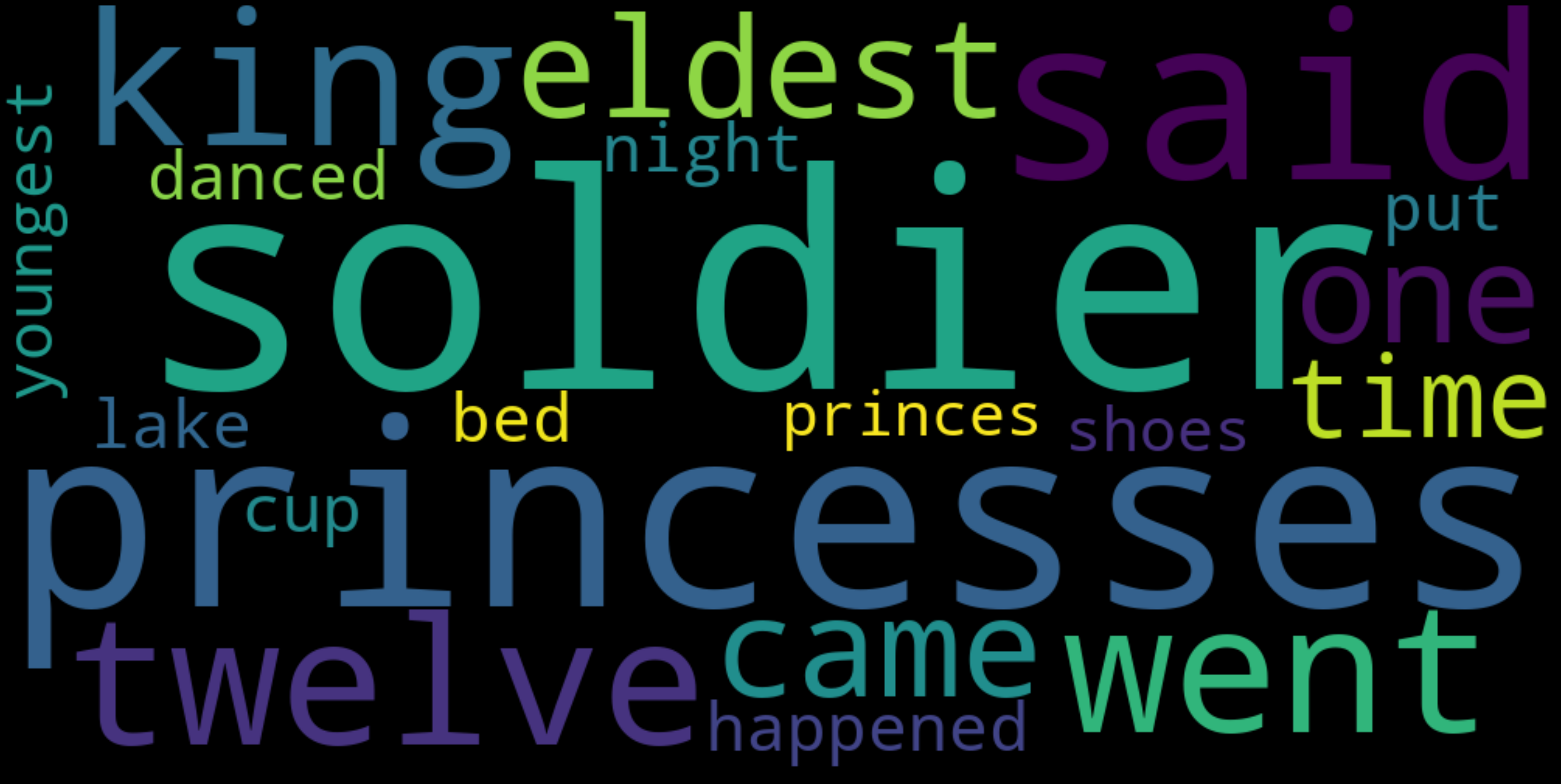
We use bilinear interpolation, this is to make the displayed image appear more smoothly. More choices can be seen here.You can chose gaussian or other options listed in the link.
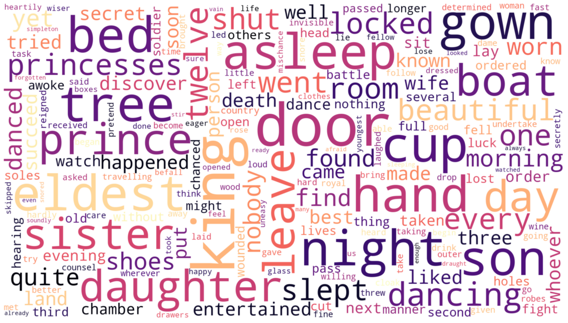
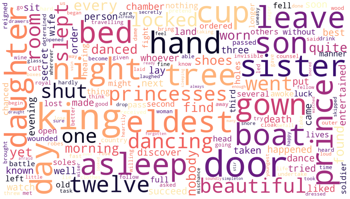
In the following code we just pass the df_fdist.Word to the code and see the cloud forming.
from wordcloud import WordCloud, STOPWORDS, ImageColorGenerator
def make_wordcloud(words):

    text = ""
    for word in words:
        text = text + " " + word

    stopwords = set(STOPWORDS)
    wordcloud = WordCloud(stopwords=stopwords,colormap="magma",width=1920, height=1080,max_font_size=200, max_words=200, background_color="white").generate(text)
    plt.figure(figsize=(20,20))
    plt.imshow(wordcloud, interpolation="gaussian")
    plt.axis("off")
    plt.show()
Words = df_fdist['Word']
make_wordcloud(Words)
from wordcloud import WordCloud, STOPWORDS, ImageColorGenerator
def make_wordcloud(words):

    text = ""
    for word in words:
        text = text + " " + word

    stopwords = set(STOPWORDS)
    wordcloud = WordCloud(stopwords=stopwords,colormap="magma",width=1920, height=1080,max_font_size=200, max_words=200, background_color="white").generate(text)
    plt.figure(figsize=(20,20))
    plt.imshow(wordcloud, interpolation="bilinear")
    plt.axis("off")
    plt.show()
Words = df_fdist['Word']
make_wordcloud(Words)
In case you are interested in saving your wordcloud image. Save the image in the img folder:
python
wordcloud.to_file("img/your_cloud.png")